
What's the Average Face?
Originally published on divergentblue.com in 2019, restored from backup. Some links to other sites may no longer work.
Note: This post was reconstructed with the help of my buddy Claude from notes, logs, emails, and other artifacts generated for this projet. The original published text is lost.
A Face in the Crowd
During an independent study at the University of Louisville, Dr. Chang showed me CelebA, a public dataset of 202,599 photos of celebrities. Every photo is cropped and aligned to the same 178×218 frame, so the eyes, nose and mouth land in roughly the same place each time. It also comes with 40 yes/no labels per photo: smiling, wearing a hat, bald, and so on.
Aligned faces made me wonder: what happens if you just average them?
The Simplest Possible Algorithm
The method really is as simple as it sounds. For every pixel position, add up the red, green and blue values across all of the images, then divide by the number of images.
for fl in filenames:
    pix = Image.open(img_root / fl).load()
    for x in range(width):
        for y in range(height):
            img_data[(x, y)] = tuple(map(sum, zip(img_data[(x, y)], pix[x, y])))

# ...then divide every pixel's running total by the number of images
There’s no danger of overflow: the biggest possible sum is 255 × 202,599 = 51,662,745, which fits in a Python int with plenty of room to spare. Memory use stays flat because only one image is ever open at a time. On my 8-core laptop the full run took about three hours, and nearly all of that was disk I/O.
Before settling on this, I tried loading every pixel into SQL Server so I could average it with a query. That file came out to about 200 GB and 7 billion rows. No thank you.
The Average Face
Here it is, all 202,599 of them at once:
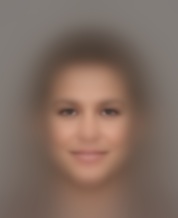
It’s a little blurry, which makes sense: the features line up because the photos are aligned, but hair, backgrounds and head tilt don’t. It still looks remarkably like an actual person.
Slicing by Attribute
The labels are where it gets fun. I loaded them into a database table and wrote one query per subgroup (WHERE Male = 1, WHERE Wearing_Hat = 1, and so on), then ran the same averaging script on each group.
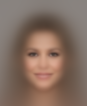
118,165 photos
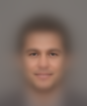
84,434
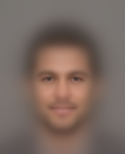
33,441
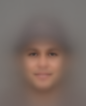
9,818
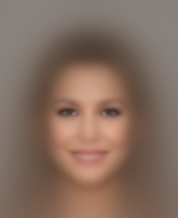
24,913
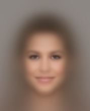
103,833
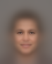
98,766
A few things jump out:
- Hats survive averaging. With fewer than 10,000 photos and a lot of different hats, you can still clearly see a brim.
- Beards do too, and the bearded average is visibly darker around the jaw than the general male average.
- Necklaces mostly mean women. The necklace average looks almost identical to the female average, because nearly everyone labeled with a necklace is also labeled female.
- “Attractive” is a loaded label. The attractive average looks almost exactly like the female average, while the unattractive average looks male. That says less about faces than about how the labels were assigned. It’s a good reminder that a model trained on these labels would learn the labelers’ biases right along with everything else.