The Story of Squaring a Triangle

A Decade Long Problem

Back in 1998, I overheard my high school math teacher musing to another teacher about the following problem:

Given a line segment of unit length, select any two points to cut the line into three parts. What is the probability that the resulting three line segments will form a “good” triangle.

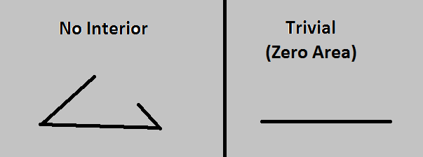By a “good” triangle, he meant one which completely encloses a non-zero area. That is, if the longest side is longer than the sum of the other two sides, it’s impossible to use those three segments to enclose an area. The trivial case exists where the longest side is equal to the sum of the shorter sides, but this triangle encloses no area.

A Delayed Response

Several years later, after I had learned to program myself, I wrote a Monte Carlo algorithm to simulate this situation, but much to my dismay, after 1000 trials, I got a probability of a little more than $.19$. To me, this certainly meant that the answer should really be $\frac{1}{5}$ - I just needed a few more trials. Unfortunately, as I increased my trial size, the number started converging to $.1931-ish$. This really disturbed me, but at the time, I was weak, so I gave up.

Renewed Strength

Many years later, in 2007, after graduate school, I decided to approach the problem from a theoretical perspective, and after some fumbling around in an attempt to create a probability distribution function, an insight from a former professor lit my path. He suggested that I think of the cuts as a two-dimensional x-y graph, where any point $(x,y)$ on the graph, represents cuts at locations $x$ and $y$ on the line segment. Let’s see what this looks like:

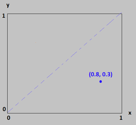Assuming the line segment is of unit length, then the two cuts, $x$ and $y$ both lie in the interval $(0,1)$. As an example, the point $(0.8, 0.3)$ would correspond to cuts at locations $0.3$ and $0.8$ on the line segment. This happens to result in a middle piece of length $0.5$, meaning that it corresponds to the trivial case of a bad triangle noted above.

This was useful because now I could analyze the graph for the regions which create good triangles, and the ones which create bad ones. I started by considering how the cuts might go awry. The simple answer is that any time one of the segments is larger than $0.5$, I get a bad triangle. This can happen, of course,  in three ways:

Segment $A$ is too large when both cuts are greater than $0.5$. This corresponds to the area bounded by the lines $x > 0.5$ and $y > 0.5$. Segment $C$ is too large when both cuts are less than $0.5$, or the area bounded by $x < 0.5$ and $y < 0.5$. The middle segment, $B$ was a little more tricky. I am looking for the region where $|x - y| > 0.5$, which really means two different areas - one bounded by $y > x + 0.5$ and the other by $y < x - 0.5$. Take a look at the result of cutting out these “bad” sections out of the graph.

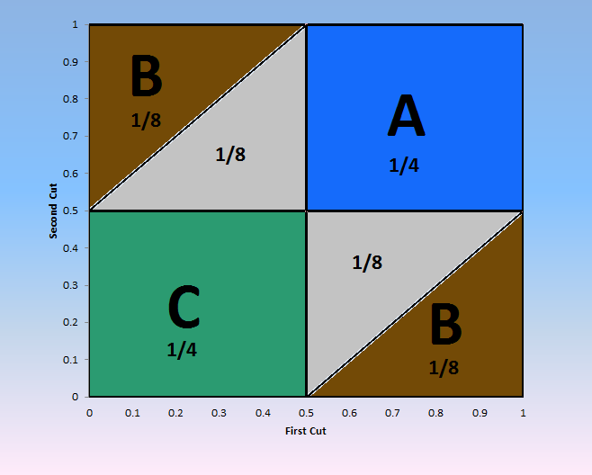The bounds described above are labeled with the corresponding line segment and I provided the value of each bounded area for reference. It was then fairly easy to see that each offending segment reduces the overall “good” area in the graph by $0.25$. In total, that leaves only $0.25$ of good area left, so this was my result. That is, one fourth of the time, the two random cuts will result in a good triangle. This is so clear from the graph that my Monte Carlo simulation must have been wrong.

Time To Get Serious

Recently, and after a few years of experience as a software developer, I decided to rewrite the simulation in C#. Whereas once it took me a full day to write, I was now able to reproduce it in a few minutes. Here is the core of my rewrite:

for (int i = 0; i < numberOfCuts; ++i)
 {
   List<double> sides = new List<double>();
   double firstCut = rng.NextDouble();
   double secondCut = rng.NextDouble();
   double lowCut = Math.Min(firstCut, secondCut);
   double highCut = Math.Max(firstCut, secondCut);
   sides.Add(lowCut);
   sides.Add(highCut - lowCut);
   sides.Add(1.0 - highCut);
   sides.Sort();
   if (sides[0] + sides[1] < sides[2])
   {
     bad++;
   }
   else
   {
     good++;
   }
 }

To my delight, after $1000000$ trials, I get $.2508$! Now I was feeling very confident about both my theoretical approach and my algorithm, so I wanted to introduce a little more complexity.

For efficiency pedants, I will concede that instead of checking the sum in the “if” condition above, I could simply check that the longest side does not exceed $0.5$, but over the course of one run of $1000000$ trials, I doubt it would make any tangible difference.

A New Challenger Emerges

To create a slightly more interesting problem, I imposed the restriction that the first cut alone is responsible for defining segment $A$. Then the second cut can only act on the line segment to the right of the first cut. How would this change the result, if at all?

Well, now that I had a working simulation, I only really needed to change one line of code to account for this new criterion. Instead of generating a random number between zero and one for the $y$ value, I simply generated a random number between the location of the first cut and one. Effectively, I was simply imposing the condition that $y > x$ for the second cut. Here’s the one-line code change:

double secondCut = rng.NextDouble();

becomes

double secondCut = firstCut + (1 - firstCut) * rng2.NextDouble();

After running this slightly modified algorithm over $10,000,000$ trials, I got a probability of $0.1933218$. But that’s almost exactly what my old algorithm gave me! I felt pretty sure I had found the bug in my original program. I had somehow implicitly assumed that $y$ must always be larger than $x$. Incidentally, after looking over my old code, I was indeed imposing that restriction by only letting the second cut act on the second piece of string created from the first cut.

To confirm the new solution, I simply calculated it the old fashioned way, primarily because the geometric solution is not nearly as obvious for this problem, which we’ll see later. Let me reproduce that logic for you:

Again, I considered the bad regions first, and ruled them out. Of course, any cut where $x > 0.5$ is disqualified because this also forces $y > 0.5$, resulting in segment $A$ being longer than $0.5$. Segment $C$ would be larger than $0.5$ when $x, y < 0.5$, so the only “good” values left fall in the range where $0 < x < 0.5$ and $0.5 < y < x + 0.5$, keeping segment $B$ from getting too large.

What is the probability of $y$ falling in this range? Well, given any particular value of $x$, let’s call it $x_{0}$, the random number generator will give me a $y$ which lies in the range $(x_{0},1)$. I am only interested in those $y$ values which lie in the range $(0.5, x_{0}+0.5)$, so the probability of this event is simply the quotient of the ranges. That is, if I define the event $G$ as $y$ taking on a value such that a “good” triangle is formed, then $P(G | x = x_{0}) = \frac{0.5 + x_{0} - 0.5}{1 - x_{0}} = \frac{x_{0}}{1-x_{0}}$.

But I’m not interested in a single value of $x$. I need to integrate over all values of $x$ to find the solution. Doing so, gives:

$\int_0^{0.5} \! \frac{x}{1-x} \, \mathrm{d} x$

And with the nifty substitution $r = 1 - x$, I get

$\int_{0.5}^{1} \! \frac{1-r}{r} \, \mathrm{d} r = [ln|r| - r]_{0.5}^1 = (0 - 1) - (ln(\frac{1}{2}) - \frac{1}{2}) = ln(2) - \frac{1}{2}$

It will probably not surprise you that this evaluates to $0.1931^{+}$, giving yet another confirmation that the simulation was a success (as well as the .NET random number generator).

One Final Piece To Explain

Now that I know the equations of the boundaries, I can look at how the graph has changed.

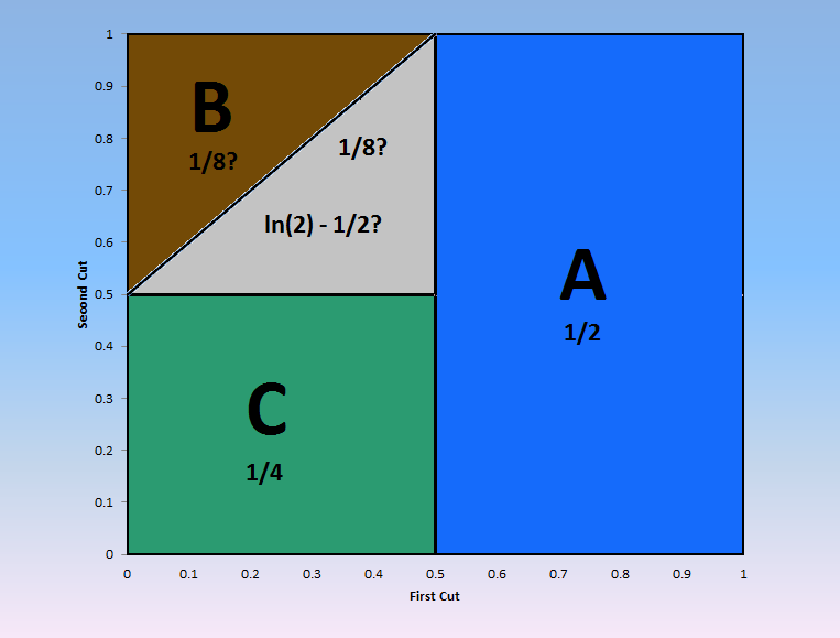
Notice that, since there is now a restriction on $x$, namely, that it must be less than $0.5$, the area which makes $A$ too large is quite big, half of the entire graph in fact. Also, note that the area corresponding to segment $C$ being too large hasn’t changed a bit. Further, all of the “good” area lies in a single contiguous region, which looks a little nicer, doesn’t it? But what about that area? It certainly looks like $\frac{1}{8}$ doesn’t it? Well, in fact, it is. Does this mean I’ve made another mistake?

As it turns out, the graph above is technically correct in that, given the stated conditions, it represents every possible pair of cuts that will yield a good triangle. The reason the actual probability is higher is simply that the distribution is no longer uniform. That is, certain points in the “good” area are actually more likely to be sampled than points in the “bad” space. This is because of the fact that an increasing value of $x$ pinches the range possible values of $y$, so that larger values of $y$ are much more likely to get sampled than lower ones. While some of these will still form a bad triangle, the ones that form a good triangle outweigh them enough to skew the probability up from $0.125$ up to almost $.2$.

What I Learned

Although it’s somewhat embarrassing that it took a student with a graduate degree in mathematics fourteen years to solve what amounts to a fairly simple probability problem, I enjoy sharing it because it reminds me of the frustration and reward of mathematics. Certainly whatever you love to do has made you feel the same, so I hope you enjoyed my story too.